
ggplotd ~master
Plotting library for the D programming library. The design is inspired by ggplot2 for R.
To use this package, run the following command in your project's root directory:
Manual usage
Put the following dependency into your project's dependences section:
GGPlotD 
GGPlotD is a plotting library for the D programming language. The design is heavily inspired by ggplot2 for R, which is based on a general Grammar of Graphics described by Leland Wilkinson. The library depends on cairo(D) for the actual drawing. The library is designed to make it easy to build complex plots from simple building blocks.
Install
Easiest is to use dub and add the library to your dub configuration file, which will automatically download the D dependencies. The library also depends on cairo so you will need to have that installed. On ubuntu/debian you can install cairo with:
sudo apt-get install libcairo2-dev
GTK Support
The library also includes support for plotting to a GTK window. You can build this in using dub with:
dub -c ggplotd-gtk
If you want to add this to link to this version from your own D program the easiest way is with subConfigurations:
    "dependencies": {
        "ggplotd": ">=0.4.5"
	},
    "subConfigurations": {
		"ggplotd": "ggplotd-gtk"
	}
Documentation
This README contains a couple of examples and basic documentation on how to extend GGPlotD. API documentation is automatically generated and put online (including examples) under http://blackedder.github.io/ggplotd/index.html. For example for the available geom* functions see: http://blackedder.github.io/ggplotd/ggplotd/geom.html
Initial examples
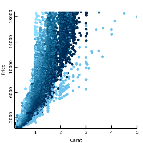
Diamonds
Let’s assume we have a csv file with data on the price, carat and clarity of different diamonds.
| carat | clarity | price |
|---|---|---|
| 0.23 | SI2 | 326 |
| 0.21 | SI1 | 326 |
| 0.23 | VS1 | 327 |
| 0.29 | VS2 | 334 |
| 0.31 | SI2 | 335 |
We can simply plot this data as follows.
import std.csv : csvReader; import std.file : readText;
import std.algorithm : map;
import std.array : array;
import ggplotd.aes : aes;
import ggplotd.axes : xaxisLabel, yaxisLabel;
import ggplotd.ggplotd : GGPlotD, putIn;
import ggplotd.geom : geomPoint;


void main()
{
    struct Diamond {
        double carat;
        string clarity;
        double price;
    }

    // Read the data
    auto diamonds = readText("test_files/diamonds.csv").csvReader!(Diamond)(
    ["carat","clarity","price"]);

    auto gg = diamonds.map!((diamond) =>
            // Map data to aesthetics (x, y and colour)
            aes!("x", "y", "colour", "size")(diamond.carat, diamond.price, diamond.clarity, 0.8))
        .array
        // Draw points
        .geomPoint.putIn(GGPlotD());

    // Axis labels
    gg = "Carat".xaxisLabel.putIn(gg);
    gg = "Price".yaxisLabel.putIn(gg);
    gg.save("diamonds.png");
}
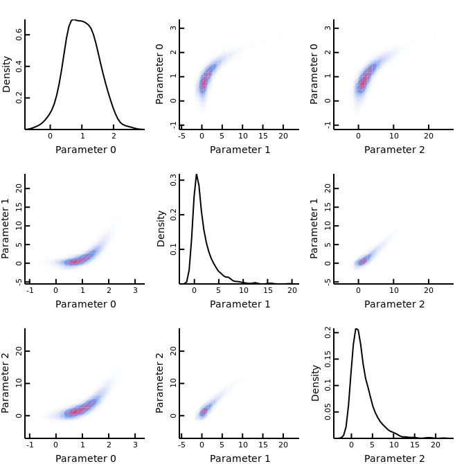
Variance-covariance
For the next example let’s assume that we have three different variables (e.g. as a result of an MCMC run) and we want to plot the variance-covariances to get a sense of how these variables/parameters relate to eachother. This could be done as follows.
import std.algorithm : map;
import std.format : format;
import ggplotd.aes : aes;
import ggplotd.axes : xaxisLabel, yaxisLabel;
import ggplotd.geom : geomDensity, geomDensity2D;
import ggplotd.ggplotd : Facets, GGPlotD, putIn;
import ggplotd.colour : colourGradient;
import ggplotd.colourspace : XYZ;

void main()
{
    // Running MCMC for a model that takes 3 parameters
    // Will return 1000 posterior samples for the 3 parameters
    // [[par1, par2, par3], ...]
    auto samples = runMCMC();

    // Facets can be used for multiple subplots
    Facets facets;

    // Cycle over the parameters
    foreach(i; 0..3)
    {
        foreach(j; 0..3)
        {
            auto gg = GGPlotD();

            gg = format("Parameter %s", i).xaxisLabel.putIn(gg);
            if (i != j)
            {
                // Change the colourGradient used
                gg = colourGradient!XYZ( "white-cornflowerBlue-crimson" )
                    .putIn(gg);
                gg = format("Parameter %s", j).yaxisLabel.putIn(gg);
                gg = samples.map!((sample) => aes!("x", "y")(sample[i], sample[j]))
                    .geomDensity2D
                    .putIn(gg);
            } else {
                gg = "Density".yaxisLabel.putIn(gg);
                gg = samples.map!((sample) => aes!("x", "y")(sample[i], sample[j]))
                    .geomDensity
                    .putIn(gg);
            }
            facets = gg.putIn(facets);
        }
    }
    facets.save("parameter_distribution.png", 670, 670);
}
Data
The initial step in plotting your data is to map the variables to
“aesthetic” variables as understood by the geom functions provided in
ggplotd. This mapping can be done using the
aes function to
map existing variable names to x, y etc. Of course if your data already
uses these variable names then this is not needed. Another useful function here
is merge, which
can be used to merge new/different mappings as in the following examples:
void main()
{
    import ggplotd.aes : aes, merge;
    struct Data1
    {
        double value1 = 1.0;
        double value2 = 2.0;
    }

    Data1 dat1;

    // Merge to add a value
    auto merged = aes!("x", "y")(dat1.value1, dat1.value2)
        .merge(
            aes!("colour")("a")
        );
    assertEqual(merged.x, 1.0);
    assertEqual(merged.colour, "a");

    // Merge to a second data struct
    struct Data2 { string colour = "b"; }
    Data2 dat2;

    auto merged2 = aes!("x", "y")(dat1.value1, dat1.value2)
        .merge( dat2 );
    assertEqual(merged2.x, 1.0);
    assertEqual(merged2.colour, "b");

    // Overriding a field
    auto merged3 = aes!("x", "y")(dat1.value1, dat1.value2)
        .merge(
            aes!("y")("a")
        );
    assertEqual(merged3.y, "a");
}
Extending GGPlotD
Due to GGPlotD’s design it is relatively straightforward to extend GGplotD to support new types of plots. This is especially true if your function depends on the already implemented base types geomType, geomLine, geomEllipse, geomRectangle and geomPolygon. The main reason for not having added more functions yet is lack of time. If you decide to implement your own function then please open a pull request or at least copy your code into an issue. That way we can all benefit from your work :) Even if you think the code is not up to scratch it will be easier for the maintainer(s) to take your code and adapt it than to start from scrap.
stat*
The stat* functions are meant to calculate different statistics from data. The results should be an range of aesthetic mappings that can be passed to a geom* function and plotted. There are a variety of existing functions (statHist, statDensity, statFunction etc.). Of course if you have written your own then you are encouraged to open a issue/pull request on github to submit them for inclusion, so that others can benefit from your good work. See below for an example of a plot created with the statFunction, which makes it straightforward to draw different functions.
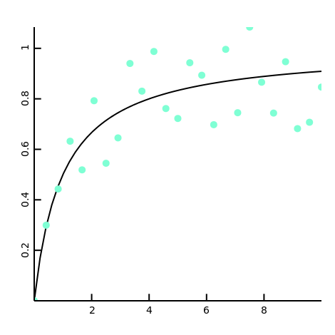
The goal of each stat funtion should be to return an aesRange that can be drawn with a variety of different geom functions. Still in many cases the results can only really be drawn in one way. In that case it might make sense to design your function in a way that is drawable by geomType. GeomType makes it easy to define the type of plot you want, i.e. a line, point, rectangle etc.
geom*
A geom function reads the data, optionally passes the data to a stat function for transformation and returns a range of Geom structs, which can be drawn by GGPlotD(). In GGPlotD the low level geom function such as [geomType](http://blackedder.github.io/ggplotd/ggplotd/geom/geomType.html), [geomPoint](http://blackedder.github.io/ggplotd/ggplotd/geom.html#geomPoint), [geomLine](http://blackedder.github.io/ggplotd/ggplotd/geom.html#geomLine), [geomEllipse](http://blackedder.github.io/ggplotd/ggplotd/geom.html#geomEllipse), [geomRectangle](http://blackedder.github.io/ggplotd/ggplotd/geom.html#geomRectangle) and [geomPolygon](http://blackedder.github.io/ggplotd/ggplotd/geom.html#geomPolygon) draw directly to a cairo.Context. Luckily most higher level geom functions can just rely on calling those functions. For reference see below for the geomHist drawing implementation. Again if you decide to define your own function then please let us know and send us the code. That way we can add the function to the library and everyone can benefit.
/// Draw histograms based on the x coordinates of the data
auto geomHist(AES)(AES aes, size_t noBins = 0)
{
    import ggplotd.stat : statHist;
    return geomRectangle( statHist( aes, noBins ) );
}
Note that the above highlights the drawing part of the function. Converting the data into bins is done in a separate bin function, which can be found in the code.
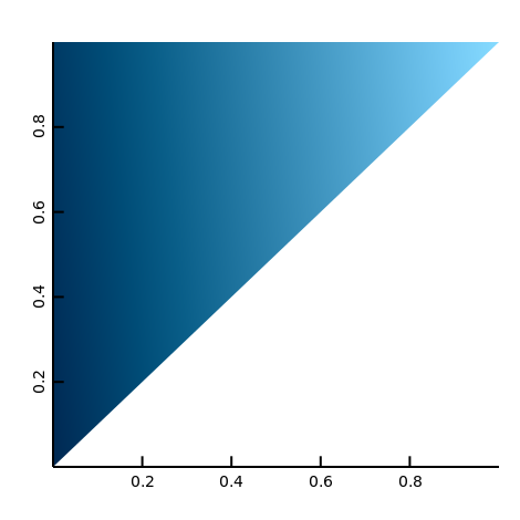
Heightmap/surface plots
Currently a couple of heightmap/surface geom* functions are implemented (geomHist2D and geomDensity2D). Both rely on the geomPolygon function to do the actual drawing. The geomPolygon function allows one to draw gradients dependent on height/colour. This function plots any straight/flat polygon, with the colour representing the height of the surface. Note that the function does not check whether the provided surface is flat. Because triangles are by definition straight it might be good to limit your usage to triangles, unless you are completely sure your polygon has no curves.
void main()
{
    import std.range : zip;
    import std.algorithm : map;
    import ggplotd.aes : aes;
    import ggplotd.geom : geomPolygon;
    import ggplotd.ggplotd : GGPlotD, putIn;

    // http://blackedder.github.io/ggplotd/images/polygon.png
    auto gg = zip([1, 0, 0.0], [1, 1, 0.0], [1, 0.1, 0])
        .map!((a) => aes!("x", "y", "colour")(a[0], a[1], a[2]))
        .geomPolygon
        .putIn(GGPlotD());
    gg.save( "polygon.png" );
}
Using custom surface type
If you want to use ggplotd to draw the plots, but keep the plot in memory, you can create an image surface and use drawToSurface to draw to it, without saving it to file.
auto width = 470;
auto height = 350;

auto gg = GGPlotD();

// Do what you want, i.e. add lines, add points etc.
// ...

// Create and draw to the surface. The cairo.Format you want probably
// depends on what you need to do with it afterwards.
auto surface = new cairo.ImageSurface(cairo.Format.CAIRO_FORMAT_ARGB32,
    width, height);
surface = gg.drawToSurface( surface, width, height );

// Use the resulting surface in your program
GTK window
If you build the library with GTK support you can show the plot in a window as follows:
void main()
{
    import core.thread;
    import std.array : array;
    import std.algorithm : map;
    import std.range : iota;
    import std.random : uniform;

    import ggplotd.ggplotd;
    import ggplotd.geom;
    import ggplotd.aes;
    import ggplotd.gtk;

    const width = 470;
    const height = 470;

    auto xs = iota(0,100,1).map!((x) => uniform(0.0,5)+uniform(0.0,5)).array;
    auto ys = iota(0,100,1).map!((y) => uniform(0.0,5)+uniform(0.0,5)).array;
    auto aes = xs.zip(ys).map!((a) => aes!("x","y")(a[0], a[1]));

    // Start gtk window.
    auto gtkwin = new GTKWindow();

    // gtkwin.run runs the GTK mainloop, so normally blocks, but we can
    // run it in its own thread to get around this

    auto tid = new Thread(() { gtkwin.run("plotcli", width, height); }).start();
    auto gg = GGPlotD().put( geomHist3D( aes ) );
    gtkwin.draw( gg, width, height );
    Thread.sleep( dur!("seconds")( 2 ) ); // sleep for 2 seconds

    gg = GGPlotD().put( geomPoint( aes ) );
    gtkwin.clearWindow();
    gtkwin.draw( gg, width, height );

    // Wait for gtk thread to finish (Window closed)
    tid.join();
}
Further examples
Histograms

void main()
{
    // http://blackedder.github.io/ggplotd/images/filled_hist.svg
    import std.array : array;
    import std.algorithm : map;
    import std.range : repeat, iota, chain, zip;
    import std.random : uniform;

    import ggplotd.aes : aes;
    import ggplotd.geom : geomHist;
    import ggplotd.ggplotd : putIn, GGPlotD;

    auto xs = iota(0,50,1).map!((x) => uniform(0.0,5)+uniform(0.0,5)).array;
    auto cols = "a".repeat(25).chain("b".repeat(25));
    auto gg = xs.zip(cols)
        .map!((a) => aes!("x", "colour", "fill")(a[0], a[1], 0.45))
        .geomHist
        .putIn(GGPlotD());
    gg.save( "filled_hist.svg" );
}
Histogram2D
A 2D version of the histogram is also implemented in geomHist2D. Note that we use another colour gradient here than the default.

void main()
{
    /// http://blackedder.github.io/ggplotd/images/hist2D.svg
    import std.array : array;
    import std.algorithm : map;
    import std.range : iota, zip;
    import std.random : uniform;

    import ggplotd.aes : aes;
    import ggplotd.colour : colourGradient;
    import ggplotd.colourspace : XYZ;
    import ggplotd.geom : geomHist2D;
    import ggplotd.ggplotd : GGPlotD, putIn;
    import ggplotd.legend : continuousLegend;

    auto xs = iota(0,500,1).map!((x) => uniform(0.0,5)+uniform(0.0,5))
        .array;
    auto ys = iota(0,500,1).map!((y) => uniform(0.0,5)+uniform(0.0,5))
        .array;
    auto gg = xs.zip(ys)
                .map!((t) => aes!("x","y")(t[0], t[1]))
                .geomHist2D.putIn(GGPlotD());
    // Use a different colour scheme
    gg.put( colourGradient!XYZ( "white-cornflowerBlue-crimson" ) );

    gg.put(continuousLegend);

    gg.save( "hist2D.svg" );
}
Box plot

void main()
{
    // http://blackedder.github.io/ggplotd/images/boxplot.svg
    import std.array : array;
    import std.algorithm : map;
    import std.range : repeat, iota, chain, zip;
    import std.random : uniform;

    import ggplotd.aes : aes;
    import ggplotd.geom : geomBox;
    import ggplotd.ggplotd : GGPlotD, putIn;

    auto xs = iota(0,50,1).map!((x) => uniform(0.0,5)+uniform(0.0,5));
    auto cols = "a".repeat(25).chain("b".repeat(25));
    auto gg = xs.zip(cols)
        .map!((a) => aes!("x", "colour", "fill", "label" )(a[0], a[1], 0.45, a[1]))
        .geomBox
        .putIn(GGPlotD());
    gg.save( "boxplot.svg" );
}
Custom axes, margins, image size and title

void main()
{
    // http://blackedder.github.io/ggplotd/images/axes.svg
    import std.array : array;
    import std.math : sqrt;
    import std.algorithm : map;
    import std.range : iota;

    import ggplotd.aes : aes;
    import ggplotd.axes : xaxisLabel, yaxisLabel, xaxisOffset, yaxisOffset, xaxisRange, yaxisRange;
    import ggplotd.geom : geomLine;
    import ggplotd.ggplotd : GGPlotD, putIn, Margins, title;
    import ggplotd.stat : statFunction;

    auto f = (double x) { return x/(1+x); };
    auto gg = statFunction(f, 0, 10.0)
        .geomLine
        .putIn(GGPlotD());

    // Setting range and label for xaxis
    gg.put( xaxisRange( 0, 8 ) ).put( xaxisLabel( "My xlabel" ) );
    // Setting range and label for yaxis
    gg.put( yaxisRange( 0, 2.0 ) ).put( yaxisLabel( "My ylabel" ) );

    // change offset
    gg.put( xaxisOffset( 0.25 ) ).put( yaxisOffset( 0.5 ) );

    // Change Margins
    gg.put( Margins( 60, 60, 40, 30 ) );

    // Set a title
    gg.put( title( "And now for something completely different" ) );

    // Saving on a 500x300 pixel surface
    gg.save( "axes.svg", 500, 300 );
}
Finally there are examples available in the online documentation. Mainly here and here.
Development
Actual development happens on github, while planning for new features is tracked on trello. Feel free to join the discussion there.
References
Wilkinson, Leland. The Grammar of Graphics. Springer Science & Business Media, 2013.
- Registered by Edwin van Leeuwen
- ~master released 4 years ago
- BlackEdder/ggplotd
- BSL-1.0
- Copyright © 2015, Edwin van Leeuwen
- Authors:
- Dependencies:
- cairod, dstats, painlesstraits, color, dunit
- Versions:
-
Show all 57 versions1.2.3 2021-Apr-12 1.2.2 2020-Dec-02 1.2.1 2020-Feb-16 1.2.0 2019-Oct-03 1.1.9 2019-Jun-26 - Download Stats:
-
-
0 downloads today
-
1 downloads this week
-
3 downloads this month
-
102283 downloads total
-
- Score:
- 2.3
- Short URL:
- ggplotd.dub.pm